资源简介
用 Matlab实现带通滤波器,对于研究带通采样定理很有好处的。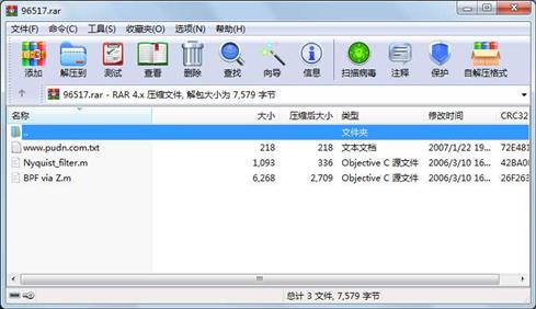
代码片段和文件信息
%Run from editor Debug(F5)
%This M file constructs a two pole two zero bandpass filter using the Z Transform
%transfer function and analyzes the characteristics of the filter such as frequency response and
%phase using the Matlab filter function with input vector x
%to get output y=filter(bax).Frequency domain plots are also provided to
%analyze the bandpass filter.
%The z transform is just basically a transformation from a linear continuous system to
%a sampled system.
%The center frequency and 3dB bandwidth(fBW) of the BPF filter can be set to
%<100Hz to >1GHz by appropriate setting of the sampling frequency(fs) and
%center frequency(fcent) and by use of the following formula(BW=(1-a)/sqrt(a)) where
%BW=2*pi*fcent/fs and (a) is the imaginary pole magnitudes. To get 0dB of attenuation
%at the center frequency(fcent)the poles must be at an angle of 2*pi*fcent/fs=pi/2.
%This corresponds to +/-j on the unit circle in the z domain. The symbolic math
%processor in Matlab is used with the “solve“ function to determine the
%value as shown typed in the command window “solve(‘2*(1-a)/sqrt(a)=BW‘)“.
%The purpose of constructing this M file was instigated by the following facts.
%I have some knowledge of Laplace transforms and the s plane. Someone mentioned
%using z transforms and I said “What is a z transform that sounds complicated?“.
%So I am trying to understand what it‘s all about. Anyway that‘s why.
%I have added references at the end of the program that I have found
%helpful and hopefully playing with the program will give you a better
%understanding of the theory. Always remember to set your axis settings on
%plot routines. The following describes the BPF.
%Bandpass filter 2 poles 2 zeros
%H(z)=(z+1)*(z-1)/(z+jp)*(z-jp)=(z^2-1)/(z^2-(p^2)
%zeros at +/-1
%pole at +j/-j
%
%                                pi/2
%                      Z plane   !+j(imag axis)
%                                x
%                     fs/2       !
%2 poles2 zeros   (-1)0---------!---------(+1)real axis
%                      pi        !
%                                x
%                                !-j
%
%
%==================================================
%Design example
%==================================================
clear
fcent=6500e6;%center frequency of bandpass filter
fBW=1000e6;%3dB bandwidth
fs=26e9;%sampling frequency(set ~4 times fcent)
%f/fs=.5set f=.5*fs
f=[0:1e6:13e9];%keep interval steps high for lower
%computer processing time
Fn=fs/2;%nyquist frequency-used in fft plots
w=2*pi*f/fs;%set so w=pi or 3.14
z=exp(w*j);%z definition
BW=2*pi*fBW/fs;
%solve(‘2*(1-a)/sqrt(a)=BW‘)%-solving for a gives a=.8862
%One could also use the symbolic math processor and construct a graph to
%solve for (a).
%type in command window the following:
%syms BW a
%BW=(2*(1-a)/sqrt(a))
%ezplot(BW)axis([0 1 0 1])ylabel(‘BW‘)grid on
a=.8862;
p=(j^2*a^2);%multiply (j*a)*(-j*a)
gain=.105;%set gain for un
属性 大小 日期 时间 名称
----------- --------- ---------- ----- ----
文件 1093 2006-03-10 16:10 Nyquist_filter.m
文件 6268 2006-03-10 16:23 BPF via Z.m
----------- --------- ---------- ----- ----
7579 3
相关资源
- matlab带通滤波器
- 数字图像处理DSP_IIR带通滤波器的设计
- DSP设计FIR带通滤波器报告&源代码
- 噪声音乐信号的巴特沃斯带通滤波器
- 基于频率采样法FIR带通滤波器设计
- 带通滤波器 Multisim仿真程序
- 带通滤波器MATLAB程序139688
- 带通滤波器matlab程序
- FIR带通滤波器源代码
- FIR带通滤波器的matlab仿真
- 压控电压源二阶有源带通滤波器 40K
- MATLAB带通滤波器程序
- matlab汉宁窗带通滤波器的设计
- 巴特沃斯带通滤波器(bandpass butterw
- 基于matlab的低通、高通、带通滤波器
- MATLAB仿真IIR带通滤波器
- 二阶 巴特沃斯 带通滤波器设计
- 基于MATLAB的FIR带通滤波器的程序设计
 川公网安备 51152502000135号
评论
共有 条评论