资源简介
关于IPIX雷达数据读取(cdf文件读取)和处理的相关程序,适用于matlab2010及更新的matlab版本,压缩文件里面有较详细程序说明。
同时,本程序还涉及海杂波的分布拟合和观测。
Provide the example of IPIX radar data reading (about CDF file) and handling, which applies to later matlab versions than 2010. There's a more detailed explanation inside the compressed file.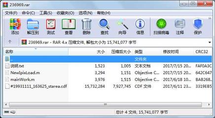
代码片段和文件信息
clc;
clear all;
close all;
%% Read the necessary data %%

file = ‘#19931111_163625_starea.CDF‘;
ncdisp(file);
finfo = ncinfo(file);
azi = ncread(file‘azimuth_angle‘);
range = ncread(file‘range‘);
data = int16(ncread(file‘adc_data‘));
N = 131072;
n = 14;
data = permute(data[4 3 2 1]);
pol = ‘vv‘; % hh hv vh vv
mode = ‘auto‘ ;% ‘raw‘ (no pre-processing)
           % ‘auto‘ (automatic pre-processing)
           % ‘dartmouth‘ (pre-processing for dartmouth files containing land)

%% If try to use the data of 93 use this part to correct the data %%

for a = 1:4
    for b = 1:14
        for c = 1:2
            for d = 1:131072
                if (data(dcba)) < 0
                    data(dcba) = data(dcba) + 256;
                end
            end
        end
    end
end


%% Normalization %%

for rangebin = 1:n
    [I(:rangebin)Q(:rangebin)meanIQstdIQinbal] = NewIpixLoad93(finfodatapolrangebinmode);
    R(:rangebin) = abs(I(:rangebin) + 1i * Q(:rangebin));
    r(:rangebin) = R(:rangebin) / max(R(:rangebin));
end

%% Data handling and image forming %%

dis = 2; % the range bin you wannt to observe

dbr = db(r(:dis));
fl = 1;
for i=1:N
    if dbr(i) >= -12
        k(fl) = i;
        fl = fl + 1;
    end
end

%% PDF Estimation %%

[fxri] = ksdensity(R(:dis)0:0.1:9.9);

z = 1e-9:0.1:(9.9+1e-9);
seta = rms(R(:dis))/sqrt(2); % Rayleigh distribution parameter estimation

A1 = mean(R(:dis)) * mean(R(:dis).^(-1)); % Weibull distribution parameter estimation
A2 = mean(R(:dis).^(2)) * mean(R(:dis).^(-2));
B1 = mean(R(:dis));
alpha = pi*A2/(sqrt(A2^2-A1^2)*A1);
beta = B1/gamma(1+1/alpha);

m2 = mean(R(:dis).^2);% K distribution parameter estimation
m4 = mean(R(:dis).^4);
v = (m4/(2*(m2^2))-1)^(-1);
b = 2 * sqrt(v/m2);

fz0 = z/(seta.^2) .* exp(-(z.^2)/(2*(seta.^2))); %Rayleigh distribution
fz1 = alpha/beta * ((z/beta).^(alpha-1)) .* exp(-(z/beta).^alpha); %Weibull distribution
fz2 = 2*b/gamma(v) .* (b*z/2).^v .* besselk(v-1b*z); %K distribution

%% CDF Estimation %%

[Ne Ri]=hist(R(:dis)100);
Fx = cumsum(Ne/N);

Fz0 = 1 - exp(-(z.^2)/(2*(seta.^2)));
Fz1 = 1 - exp(-(z/beta).^alpha);
Fz2 = 1 - 2/gamma(v) .* (b.*z/2).^v .* besselk(vb*z);

%% Picture %%

t = 0.001 : 0.001 : (N/1000);
mesh(rangetR);
title(‘杂波总览‘);
xlabel(‘距离(m)‘);
ylabel(‘时间(s)‘);
zlabel(‘杂波幅度‘);
grid on;

figure
stem(tr(:dis)‘marker‘‘none‘);
title(‘确定距离单元杂波分布‘);
xlabel(‘时间(s)‘);
ylabel(‘归一化杂波幅度‘);
grid on;

figure
stem(tr(:dis)‘y‘‘Linestyle‘‘none‘);
title(‘尖峰识别‘);
xlabel(‘时间(s)‘);
ylabel(‘归一化杂波幅度‘);
grid on;
hold on stem(t(k)r(kdis)‘k‘‘Marker‘‘none‘)

figure
plot(RiFx);
axis([0 10 0 1]);
title(‘CDF‘);
xlabel(‘幅度‘);
ylabel(‘累计概率‘);
grid on;
hold onplot(zFz0‘:‘);
hold onplot(zFz1‘-*‘);
hold onplot(zFz2‘--‘);
legend(‘杂波数据‘‘Rayleigh‘‘
属性 大小 日期 时间 名称
----------- --------- ---------- ----- ----
文件 15732284 2017-06-11 23:12 #19931111_163625_starea.cdf
文件 3976 2017-06-18 10:46 mainWork.m
文件 3294 2017-07-15 20:24 NewIpixLoad.m
文件 1523 2017-07-15 20:58 说明.txt
----------- --------- ---------- ----- ----
15741077 4
- 上一篇:数据处理MATLAB 算法
- 下一篇:电力系统3机9节点暂态仿真
 川公网安备 51152502000135号
评论
共有 条评论